The universe doesn’t give up its secrets easily. Every time we learn some truth, we depend on prior, equally hard-won knowledge, and usually some luck. The easy truths are getting rarer, so the excitement around speeding up science with deep learning models is understandable, especially after LLMs surprised us by learning so much just from predicting text. Today’s frontier LLMs are trained on almost the entirety of human scientific output. So why haven’t they transformed our understanding of the universe? And why is AlphaFold, a deep learning model for predicting protein structures (and very much not an LLM), one of only a handful of models to have transformed science? Why aren’t there more AlphaFolds?
The answer hinges on the difference between training models on human-generated text, which is itself downstream of knowledge acquired the hard way, and training them on observations at the limits of science where the definitive text is yet to be written. It’s easiest to see this by studying the process of scientific discovery. So let’s start by looking at two examples, with the first being the story of one of the most deadly diseases of the age of discovery: scurvy.
Scorbutic and Confused
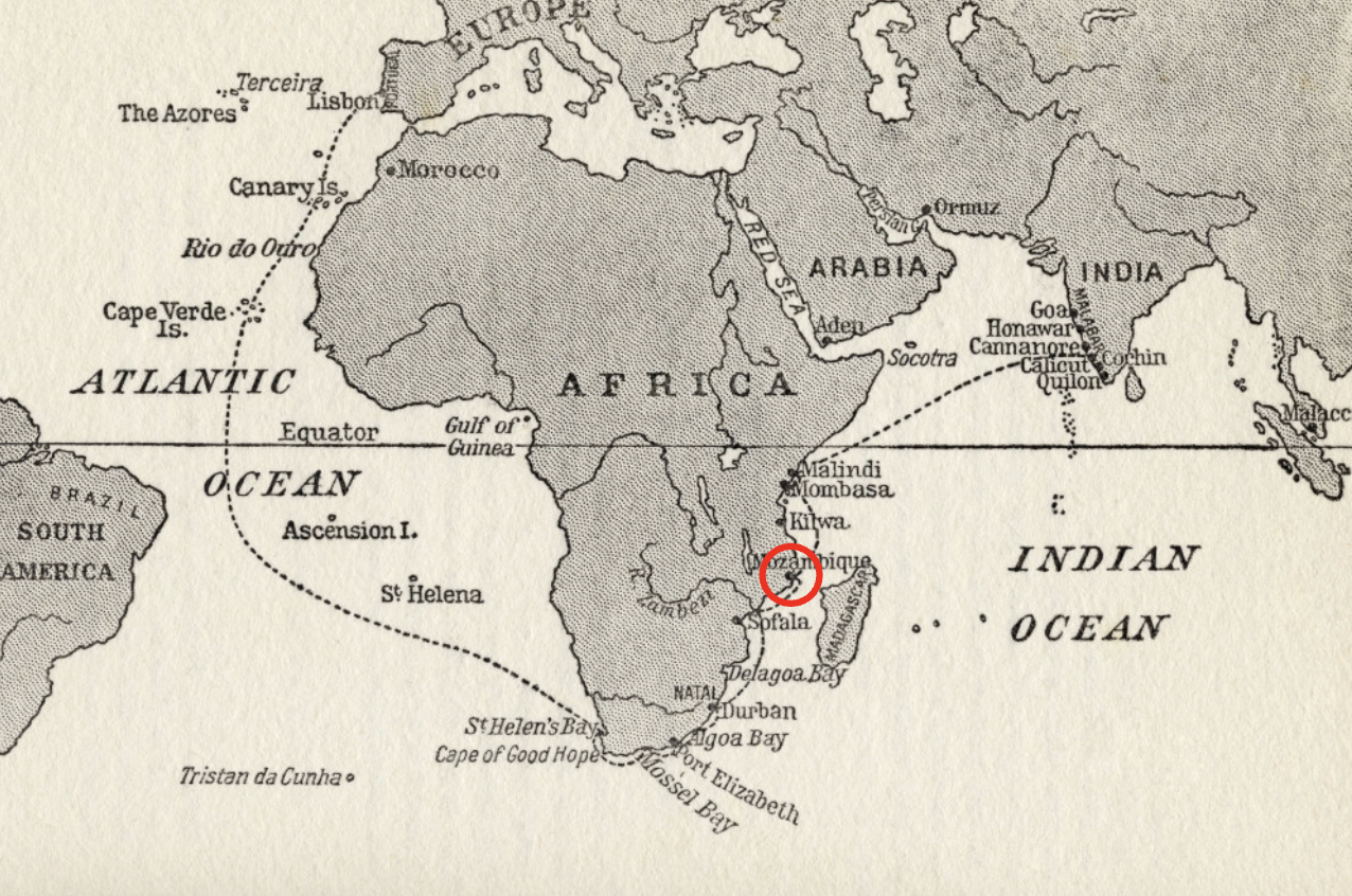
On July 8th 1497, the Portuguese mariner Vasco da Gama sails from Lisbon to find a path from Europe to India via sea, commanding an armada of four ships and 170 crew. Six months later, in January 1498, after sailing deep into the South Atlantic Ocean in search of westerly winds, they arrive at the Mozambique coast near Quelimane. The ships’ journal1:
“Many of our men fell ill here, their feet and hands swelling, and their gums growing over their teeth, so that they could not eat.”
We know what’s happening to these sailors. Their vitamin C reserves are depleted after six months at sea eating salted meat and dried crackers. You need vitamin C (amongst other things) to keep collagen intact, which is needed to keep your gums attached to your jaw. Without it, you get scurvy.
Three months later, the armada sails into Malindi (modern-day Kenya). Local trading craft approach the ships. Here’s the journal again:
One was laden with fine oranges, better than those of Portugal
Five days later, the sick miraculously recover:
“… on arriving at this city all our sick recovered their health, for the climate (“air”) of this place is very good…”
It was the “climate”, not the tasty oranges the crew ate right before they got better. To be fair to them, all the novelty they encounter sailing into Malindi confounds exactly what cured them. But as we’ll see later, attributing malady and recovery to the climate isn’t uncommon for the era.
The armada keeps going, crossing the Arabian Sea and reaching India, becoming the first Europeans to do so by sea. The same crossing on the way back takes three months against the monsoon. Half the remaining crew die. The rest limp back to Malindi, each ship having only seven or eight men left fit for duty. The journal again:
“The captain-major sent a man on shore with these messengers with instructions to bring off a supply of oranges, which were much desired by our sick.”
Despite not knowing anything about vitamins or collagen, the crew remembered the oranges, asking for them explicitly. By the time the crew returns to Lisbon, half the original crew of 170 are dead, many from scurvy.
Two hundred and fifty years later, in 1747, the Scottish physician James Lind runs one of the first controlled clinical trials2. On the HMS Salisbury, Lind gives twelve sailors with scurvy six different treatments, including oranges and lemons. Unsurprisingly, the citrus do really well. Lind writes in A treatise of the scurvy, in three parts:
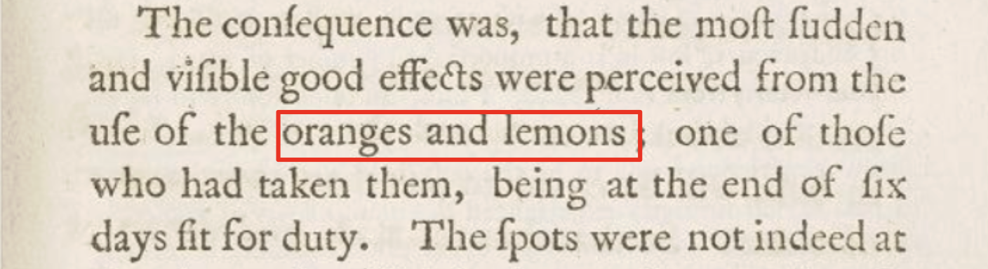
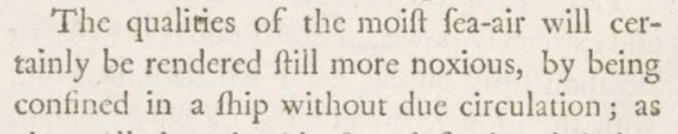
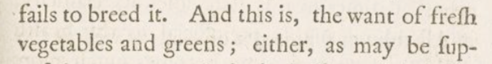
What does Lind conclude after the experiment? That scurvy is caused (amongst other things) by the “want of fresh vegetables and greens” and by the “moist sea air … rendered still more noxious, by being confined in a ship without due circulation”. Remember this diagnosis? Da Gama’s crew came to the same conclusion in Malindi. Lind’s subsequent advice to the navy to keep ships ventilated and provide fresh vegetables does nothing to prevent scurvy.
And what of the oranges and lemons that had such a positive effect? Lind instructs to preserve them on long journeys (before the invention of refrigeration) by boiling them into a “rob”:
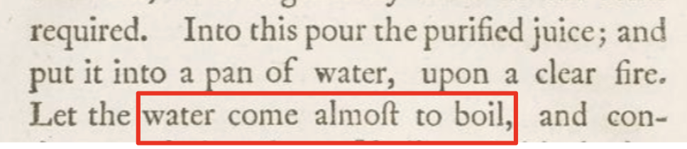
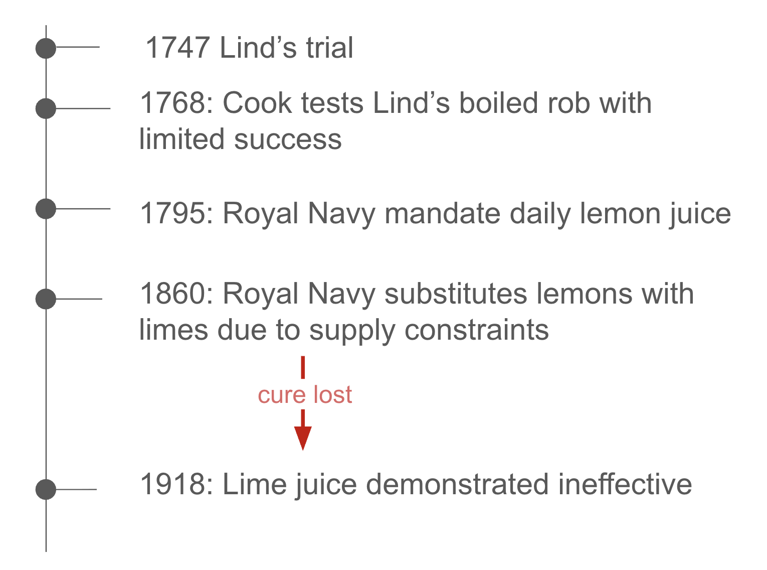
What Lind didn’t know was that boiling the juice destroys all its vitamin C. Unsurprisingly, when Captain James Cook tries Lind’s boiled rob twenty years later in 1768, he finds it lacking. Eventually the citrus signal becomes too hard to ignore and in 1795 the Royal Navy mandates daily lemon juice for sailors, eradicating the disease. But no one knows how it works, so by 1860, when lemon supplies become constrained, the Royal Navy switches to limes which don’t have as much vitamin C, and scurvy is back once again.
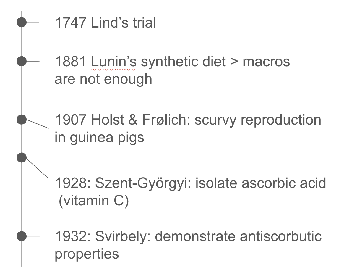
It takes nearly two centuries after Lind’s trial to piece everything together. First, Nikolai Lunin performs synthetic diet trials in 1881 which enable the discovery of vitamins. Then in 1907, Holst & Frølich accidentally induce scurvy in guinea pigs (which like us, don’t produce their own vitamin C). In 1928 Szent-Györgyi isolates vitamin C (ascorbic acid), and finally in 1932 Svirbely identifies it as the compound which prevents scurvy. The better part of two centuries too early in 1747, Lind had no chance to get the story right.
How Many Ways to Fit a Curve?
Our next story is inspired by Terence Tao’s upcoming book, and starts in 1576, when Danish astronomer Tycho Brahe convinces his patron king to build him the largest ever naked-eye observatory. This is a big deal, since the first telescope wouldn’t be invented for another 30 or so years.
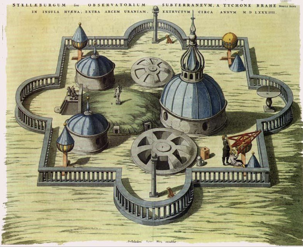
Over the next 20-something years, Brahe builds up the largest and most precise dataset of the positions of the five known planets in the sky. Tycho presumably knows about the Copernican Revolution that began in 1543, but nevertheless believes the sun orbits earth, so he’s not able to explain the observations.
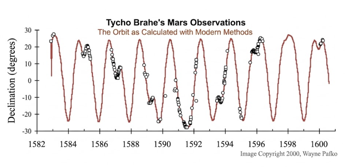
After Brahe dies, Kepler gets the dataset. After a few creative tricks of trigonometry to compute the period and distance of each planet from Brahe’s azimuth/elevation data, he arrives at six data points. To these he fits a curve explaining each planet’s orbital period using its orbital distance (really the semi-major axis) around the sun. We know this as Kepler’s third law:
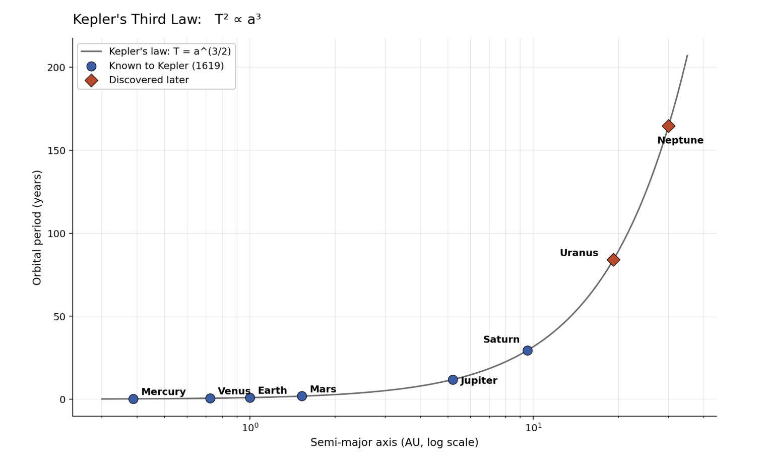
How does Kepler do it? Consequential priors. Like Copernicus, and unlike Brahe, Kepler believes the planets orbit the sun. His study of music biases him to relate orbital periods with orbital distance. And he cares about precisely explaining what he observes. Here’s Kepler on the eight arc-minute (about a tenth of a degree) discrepancy between Tycho’s Mars observations and those predicted by fitting a perfectly circular orbit to them:
these eight minutes alone will lead us along a path to the reform of the whole of astronomy
Because he cares about the cause, he’s not content with planets just moving on their own around the sun. He proposes an “immaterial emanation” pushing them along, radiating from the sun and weakening with distance, a kind of proto-theory of gravity some 70 years ahead of its time. Of course this isn’t exactly how gravity works, but it’s just right enough to lead to the correct inference.
Around 150 years after Kepler publishes his law, a German astronomer named Johann Bode proposes a different fit to the data, inspired by a proposal by the astronomer Johann Titius six years earlier. Unlike Kepler’s third law, Bode’s law discards the orbital period entirely. To Bode, each body in the solar system inhabits an orbit at a distance according to its order from the sun, starting with Mercury. To fit the data, Mars takes fourth place with Jupiter in sixth, leaving a spot between them. Bode suggests there should be a planet there. Not long after, Uranus is found in exactly the predicted distance. This causes great excitement about the predicted planet in the gap between Mars and Jupiter. Then, Ceres is discovered, right on the curve in position five.
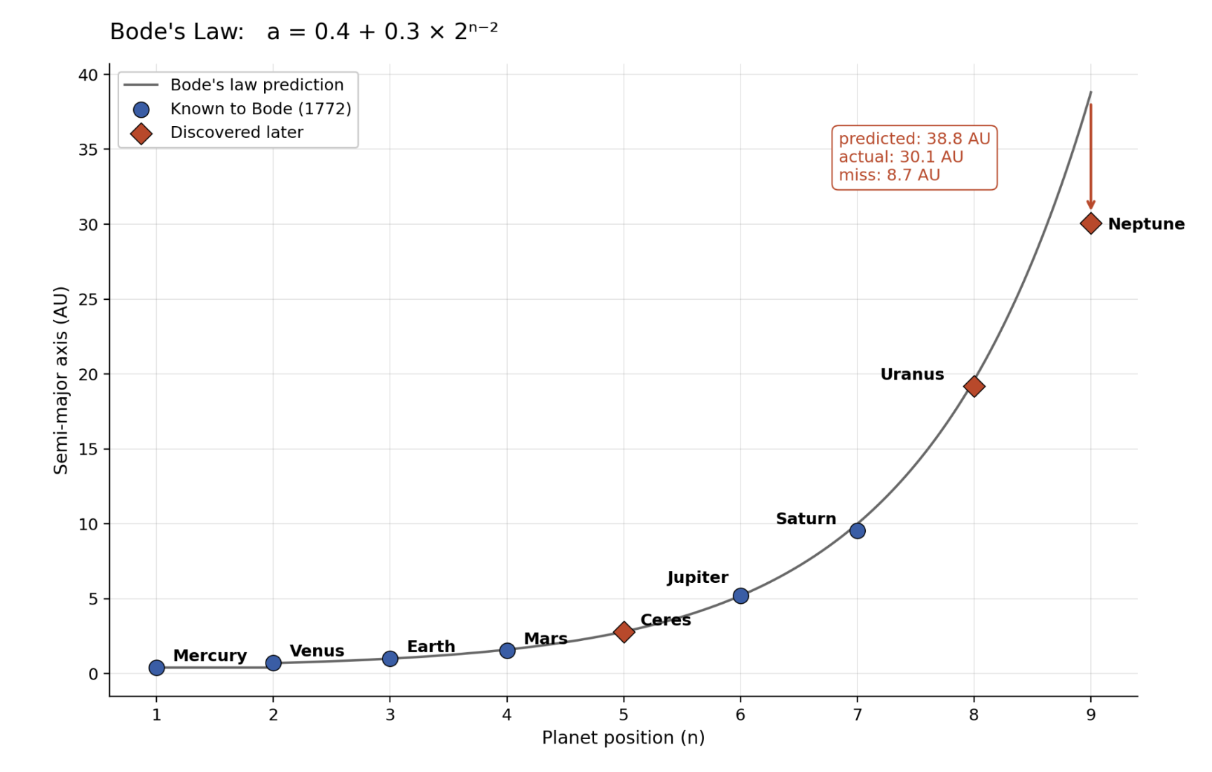
All this happens after Kepler proposes his law and Newton states the gravitational laws in Principia. Bode’s confidence is admirable: 150 years after the problem is essentially solved, he conjures an alternative explanation, one that actually makes correct predictions through sheer luck, yet completely fails to predict Neptune (which Bode does not live to see). Why did Bode do this? Our clue is in a footnote Titius sneaks into one of his translations about the vacant spot where Ceres is later found:
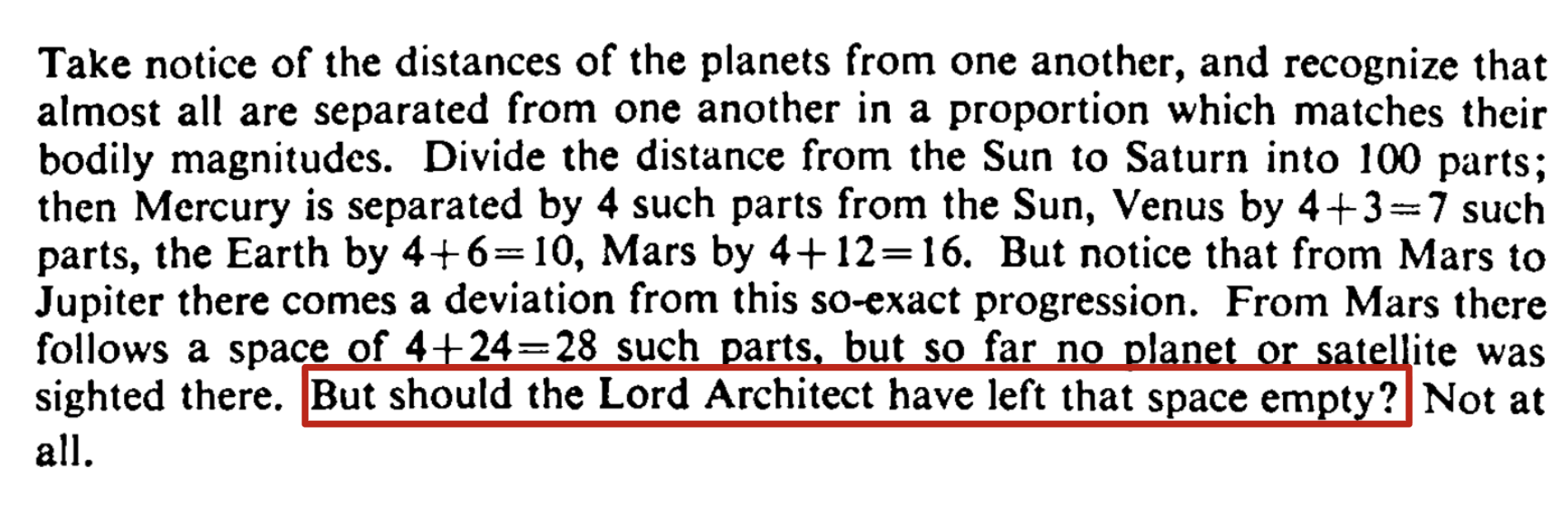
Like Kepler, Titius and Bode held aesthetic and theological priors. To them, there is an implicit order to the universe, derived from a creator. But unlike Kepler, Titius and Bode needed no further causes for the phenomena they observed.
AlphaFold’s Many Inductive Priors
In each story, someone suggests a hypothesis to explain a few hard-earned data points. They’re at the edge of human knowledge where the data comes with no explanations. They interpret what they see solely through the lens of their prior beliefs. Sometimes these beliefs are wrong (the sun revolves around the earth), luring them away from the truth. But sometimes, often with a little luck, they’re able to make leaps in understanding well ahead of their time. ML models at the frontier of human knowledge are no different, and the canonical example for this class of models is AlphaFold.
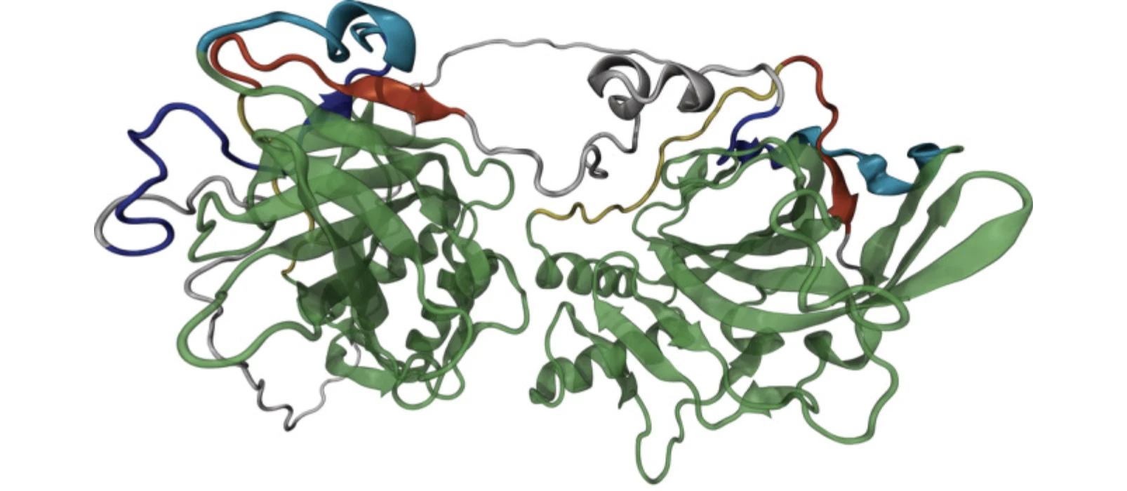
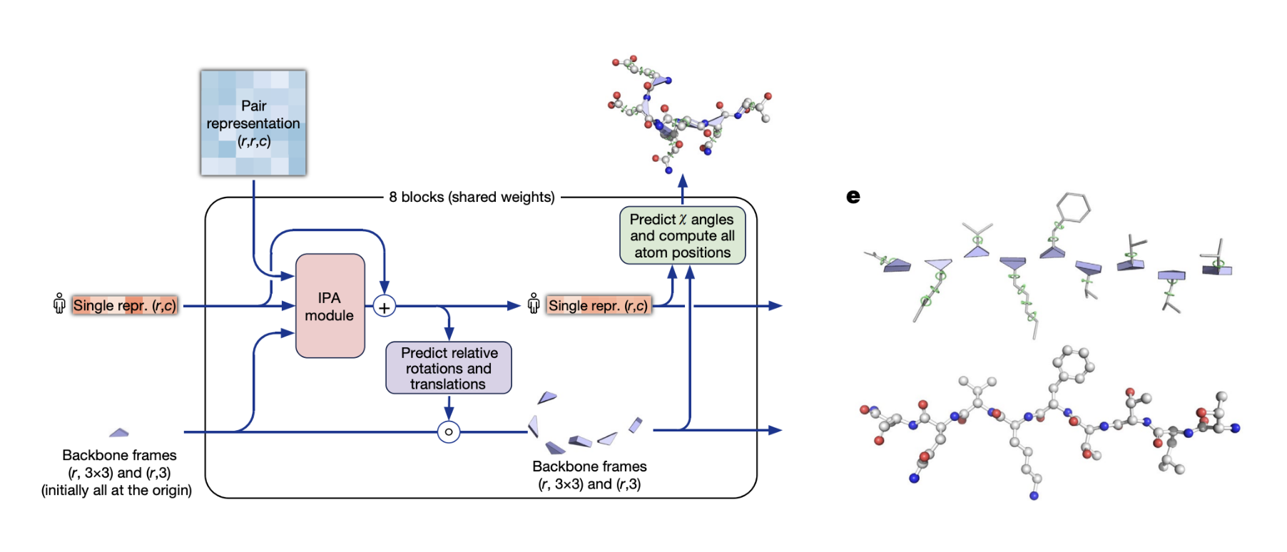
AlphaFold is a deep learning model that predicts the 3D structure of a sequence of amino acids once it is folded by the molecular machinery of the cell. The protein’s function is largely a product of its structure, so AlphaFold has been broadly impactful across molecular biology.
AlphaFold’s model architecture has similarities to modern LLMs, which are all variants of 2017’s transformer architecture. But what’s unique about it is combining the attention mechanism from transformers with specialized modules that encode prior knowledge of the protein-folding problem (inductive priors) directly into the architecture.
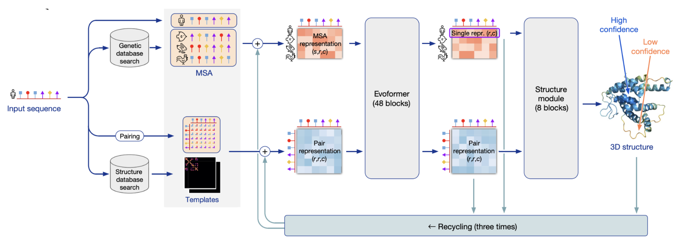
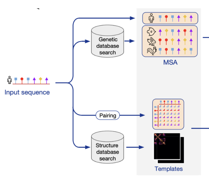
When predicting the structure of a target sequence, AlphaFold considers it together with evolutionary relatives called homologs. Why not just use the target directly? Because AlphaFold’s designers knew that residues that physically contact each other in the protein’s structure will co-evolve (if one side of the contact mutates, the other side must also mutate to compensate or it will be filtered out via selection). Looking at a target together with its homologs reveals this co-evolutionary signal. The model didn’t have to learn this domain-specific trick from scratch using the scarce PDB data because the designers baked it in as an inductive prior.
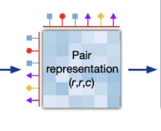
Even after considering the target and its homologs, inductive priors shape how AlphaFold represents the target sequence. The shape of a folded protein is the product of the forces residues impart on each other, so AlphaFold’s architecture explicitly encodes this by forcing the model to represent the pairwise effect of each residue on all others. Residues that are physically close in the folded structure may be nowhere near each other in the sequence, so this pairwise representation ensures that the model considers interactions between all residues, no matter how far apart in the sequence.
Even the way AlphaFold predicts the coordinates of each residue is specialized. Rather than working with global 3D coordinates, AlphaFold is instead trained to predict the coordinates of each residue relative to its neighbors. This trick focuses the prediction problem into a local space, no matter where the prediction lies on the eventual complicated 3D shape. The resulting “gas” of disconnected residues is assembled afterwards, followed by an energy minimization step that corrects outputs that may violate physics (like atoms that intersect one another).
Why does AlphaFold need all of these inductive priors? Why couldn’t it use the ubiquitous transformer architecture? The clue is in the training data. AlphaFold was trained to predict the structures of the sequences in the PDB (Protein Data Bank), a dataset of roughly 200k amino acid sequences and their 3D structures. If AlphaFold is the internal combustion engine, the PDB is the oil. It took over fifty years and tens of billions of dollars to collect the structures in it using techniques like X-ray crystallography and cryo-EM. But that’s all there was, so AlphaFold had to extract everything that could be learned from the data, and it wasn’t much.
To put just how little data AlphaFold was trained on into perspective, let’s compare its data per model parameter ratio to other recent models:
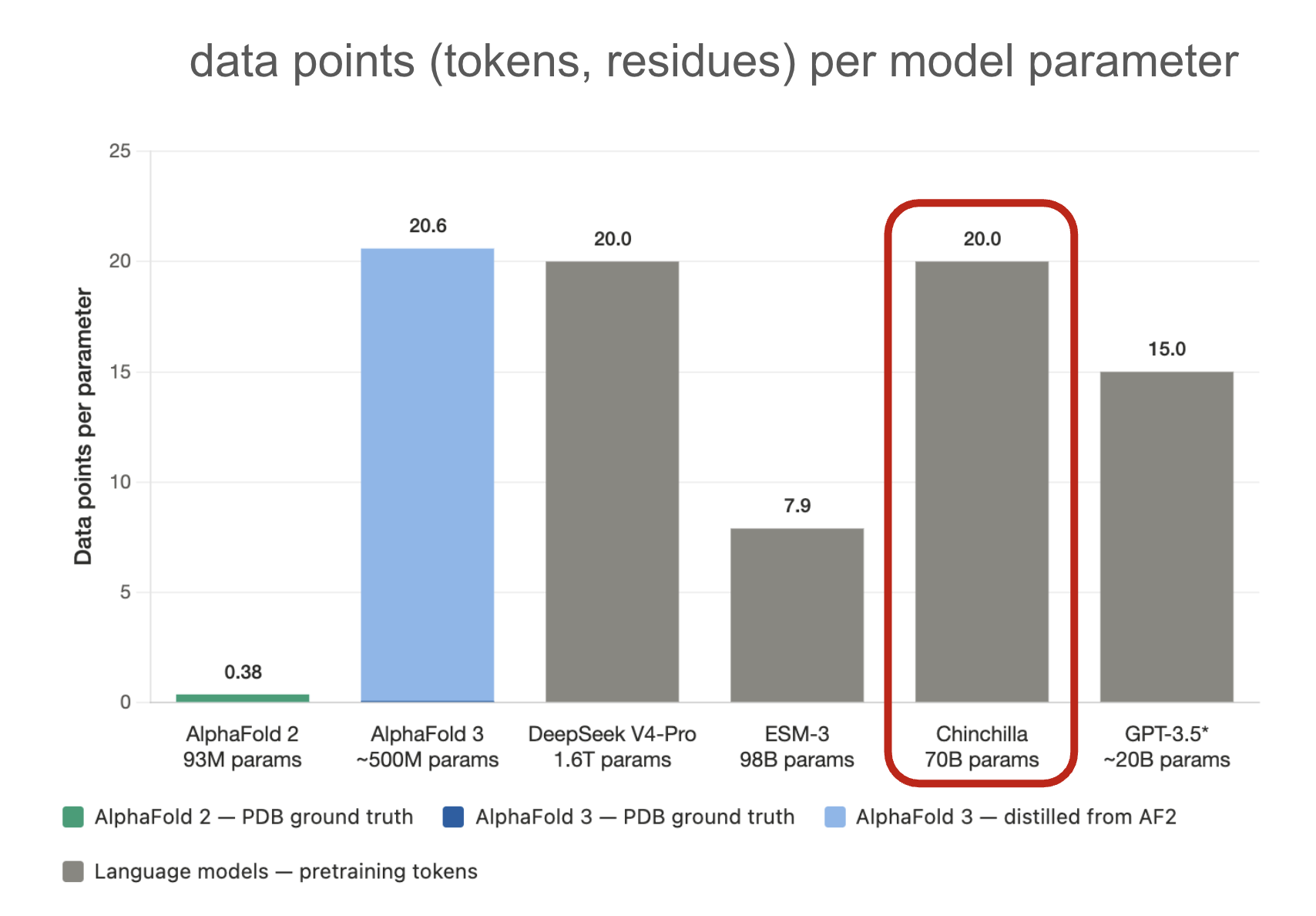
Circled in red is the compute-optimal ratio of 20 tokens per model parameter for training LLMs, published in the Chinchilla paper3. AlphaFold is at 0.38. That’s partly why it needs so many inductive priors in its architecture. Its successor, AlphaFold 3, does reach the 20:1 ratio, but only by bootstrapping off of its predecessor’s predictions. The PDB share of its dataset is so small it’s barely visible in the graph.
But there’s another more important reason AlphaFold needs so many inductive priors: Chinchilla and the frontier LLMs are trained on text, but AlphaFold is trained on the actual physical observations of sequences and the structures they fold into. The distinction matters because text is the end product of humans having already made sense of raw observations. Text doesn’t even have to be scientific or educational to have this quality. Let’s say you’re reading a Reddit thread of people arguing over what cheese works best in salad. They’ll use words like “easy to melt”, “crumbly”, or “smelly” that are grounded in an understanding of the physical qualities of cheese and how it interacts with other ingredients. These same words correlate with other texts written about similar qualities or physical interactions. When we train a model on a large enough corpus of text, it can extract a simulacrum of this web of human understanding.
When we train models on raw observations, we get none of this. We just get the raw physical measurements, and everything else, including understanding the physical mechanisms behind the measurements, is the model’s responsibility. A model trained on Brahe’s raw measurements of azimuth and elevation has to retrace Kepler’s steps to uncover the underlying dynamics of the solar system. Otherwise it will resort to memorization and won’t generalize outside the training distribution.
So one of the reasons we don’t have more AlphaFolds is that at the frontiers of knowledge, data is scarce, and unlike text, it’s mostly raw observation without any explanation. There’s no learning-from-scratch from a handful of measurements. You need to bake the prior knowledge in, AlphaFold style, which isn’t easy because you need expertise across two domains: the science domain and machine learning model design.
The Bitter Lesson
But what if we have much more than a handful of observations? Doesn’t the bitter lesson tell us that general methods (without human-engineered inductive priors) are more effective, and we should let them learn from data rather than engineering priors into them? If we could do that, we could train AlphaFolds on all sorts of hard scientific problems.
It turns out AlphaFold 2 has a successor, AlphaFold 3, which gives us a partial answer with its much larger training dataset, expanded with predictions (although down-weighted compared to PDB data) made by AlphaFold 2 on sequences without structure labels. This bootstrap trick generated massive data and let AlphaFold 3 replace some inductive priors with more general architecture design.
So what happens at the limit? If we have an unlimited supply of data, should we expect general-purpose architectures to learn the underlying mechanisms explaining that data? If yes, could these models then make correct predictions outside of the training distribution? An ideal experiment for answering this question churns out unlimited observations that are hard to memorize directly, but easy to explain with a few simple mechanisms. It’s hard to cheat without memorization. Any successful model needs to figure out something about the mechanisms.
Predicting n-body dynamics checks all the boxes we need. Observations come free with simulation, the underlying dynamics (laws of gravity) that explain them are simple, and chaotic motion makes memorization impossible. As a bonus, we get to play in Kepler’s playground. Depending on how the bodies are initialized, their motion could be stable or chaotic:
We’ll now train a few different architectures to predict 3-body motion. For all models, the training loss will be the position and velocity mean square error (MSE), aggregated over a 10-step prediction starting from each ground-truth position in the trajectory. We normalize model inputs to be relative to the center of mass, an inductive prior that stops quantities from blowing up as the bodies move away from the origin. We’ll train a range of models from those with few inductive priors such as the vanilla multilayer perceptron (MLP) or transformer, to those with problem-specific inductive priors like the MLP with a physics loss, a neural network to predict motion by representing the hamiltonian, and a graph neural network (GNN) that explicitly represents the pairwise effect of the bodies on each other. We’ll configure the models to all have the same number of parameters:
| Model | params | Configuration | Inductive priors |
|---|---|---|---|
| transformer | 36,522 | d=36, n_heads=4, n_layers=2, ctx_len=8 | |
| mlp | 37,001 | d=128, n_layers=3 | |
| physics loss mlp | 37,001 | same as mlp | energy conservation loss |
| hamiltonian mlp | 35,969 | same as mlp | model computes hamiltonian, derivatives give velocities |
| gnn | 38,774 | n_nodes=3, d_node=40, d_msg=32, num_layers=2, n_messages=3 | pairwise message-passing between bodies |
Since data is free, we’ll train with 20M samples across 100k 10-second trajectories, giving us around 500 samples per parameter. We’ll filter trajectories that have large motion nonlinearities caused by close approaches of the bodies. We want our models to learn generalized dynamics in constant time steps, and forcing them to predict the nonlinear dynamics of close approaches will pollute the learning signal.
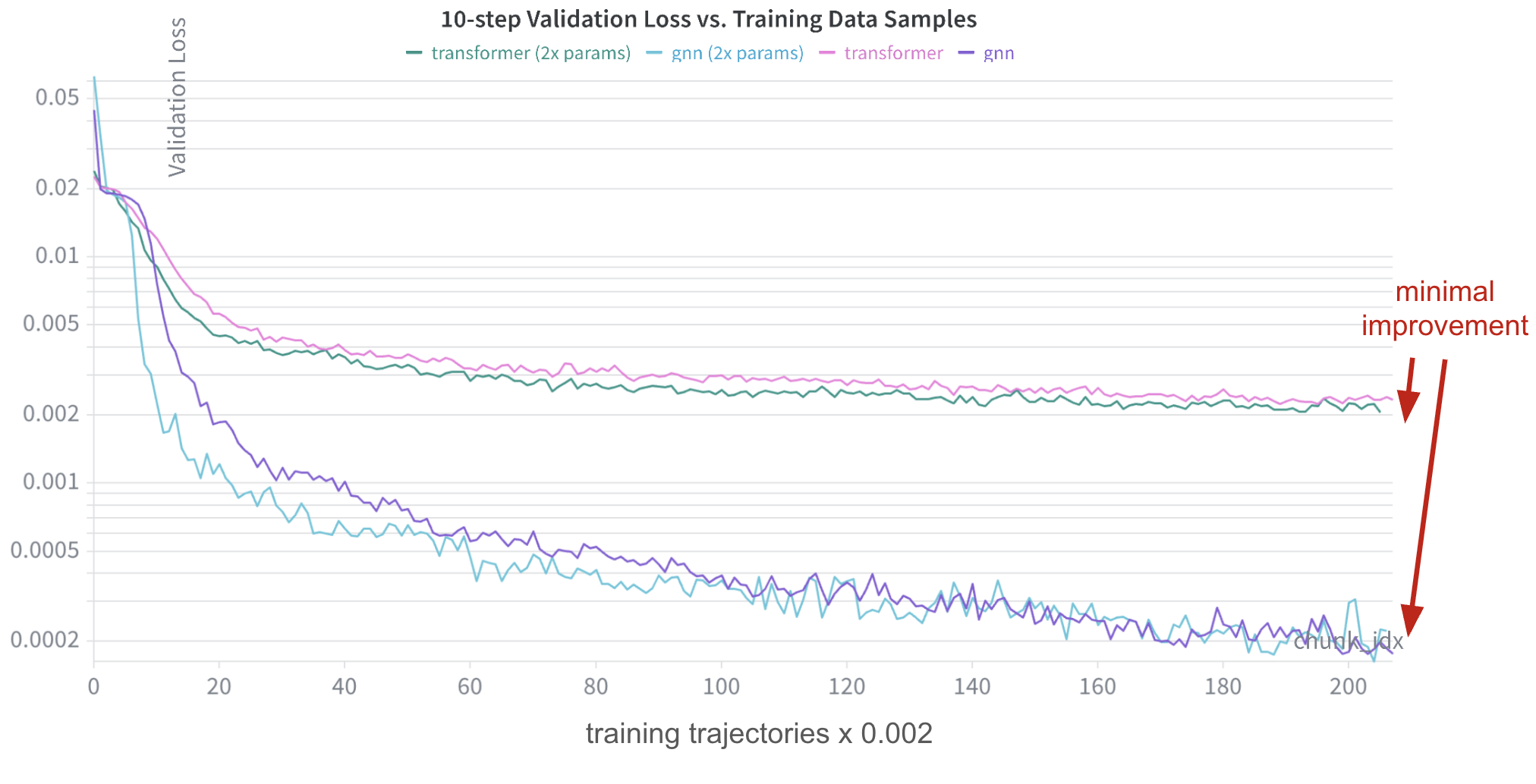
We’ll train the collection of architectures over the full 20M dataset with the AdamW optimizer, weight decay, and annealed/decayed learning-rate scheduling. It’s clear from the validation results during training that even though it lags the other architectures at the start, the GNN pulls away from the others, including even those with strong physics-specific priors. One reason could be that the GNN inductive prior that explicitly represents the pairwise effect of bodies on each other is difficult for the other models we trained to learn, even in this setting with essentially unlimited data.
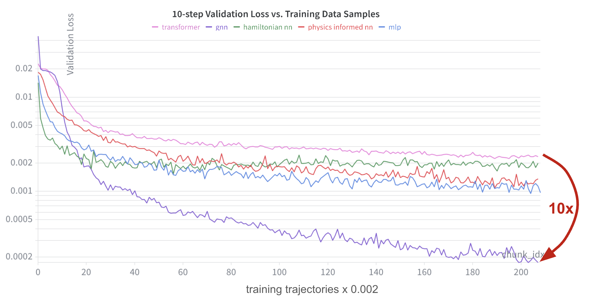
The validation loss in the graph above mirrors the training loss: aggregate position and velocity error over a 10-step prediction window, starting from each ground truth position. It represents a local measure of the model’s prediction accuracy. But what if we predict whole trajectories starting from the initial conditions? And what if we go beyond the 10 second horizon that we trained over? If the model learned generalizable dynamics, we expect consistent performance over time. We’ll use position mean square error (MSE) and total energy drift (measured as RMS of hamiltonian drift over the trajectory) as our error metrics. As expected, the GNN wins easily.
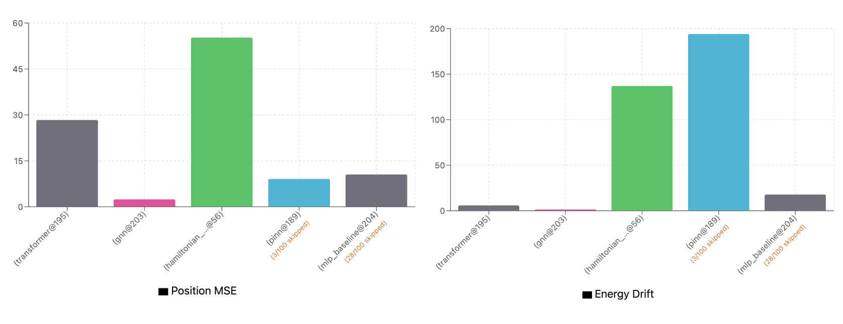
Visualizing the predictions gives us some more clues. The GNN’s predictions resemble gravitational motion even though they diverge from the ground-truth early on in the rollout. But the transformer’s predictions look completely wrong. The red and blue bodies wiggle by themselves in empty space and the green body U-turns away from the ground-truth. The transformer’s wiggle predictions look like it’s memorized the shape of orbits seen in the training data, but applied them incorrectly to single bodies rather than as a relationship.
It’s surprising that the transformer architecture does not perform better. As the architecture behind all major modern LLMs, and even models that operate on continuous data like pixels (such as vision-language or vision-language-action models), it has a proven track record. Perhaps the transformer needs more parameters to learn the pairwise representation that the GNN gets for free via inductive priors?
So We Just Need More Data?
The Kolmogorov complexity of a constant-time 3-body dynamics integrator is low (on the order of 10³ bits if using C). Nevertheless, the model may need many more bits’ worth of parameters to represent the same functions, for example because multiplicative functions are difficult to learn without specialized structures built into the architecture4. Training larger models on the same data should tell us whether model size is the bottleneck. Let’s 2x all the models and retrain.
The full five-model loss comparison is hard to read, so I’m showing only two model loss curves: GNN representing the strong-inductive-prior team, and transformer representing the (mostly) inductive-prior-free team. There’s not much of a trend line. The loss tracks mostly the same. What about evaluation over the validation dataset?
Even though the 10-step validation loss didn’t move much, position error and energy drift stability over the full validation set improved for most models other than the GNN. So perhaps they were capacity constrained after all. Let’s expand the transformer to 1M parameters and retrain. We’ll train on 3x the data (over 60M samples) to ensure the ratio of data points to model parameters stays well over 20.
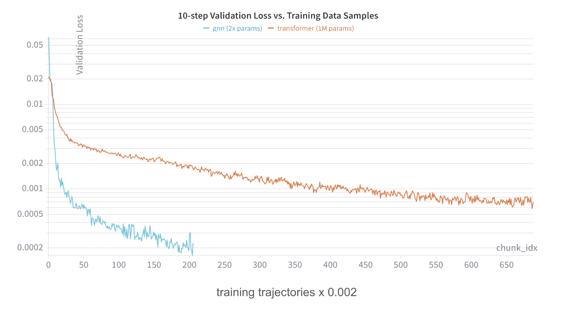
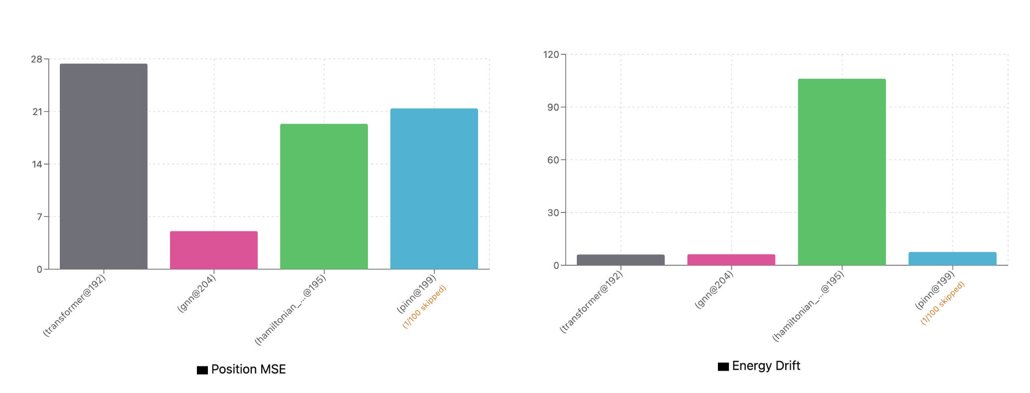
After we run the training until the transformer plateaus, the GNN still maintains a lead in the 10-step validation loss metric that mirrors our training loss. But we saw earlier that performance on the 10-step metric doesn’t map monotonically to full trajectory predictions beyond the 10 second training time horizon. So how does the 1M parameter transformer perform when predicting the entire 30 second validation trajectories?
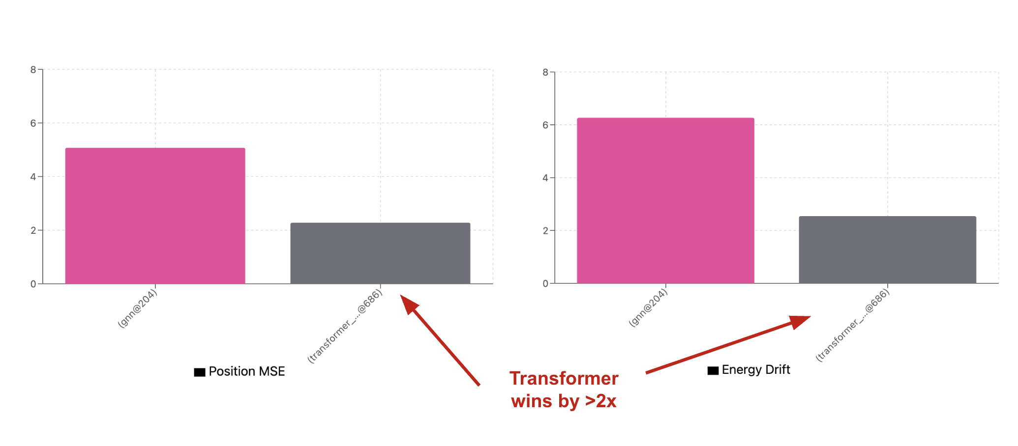
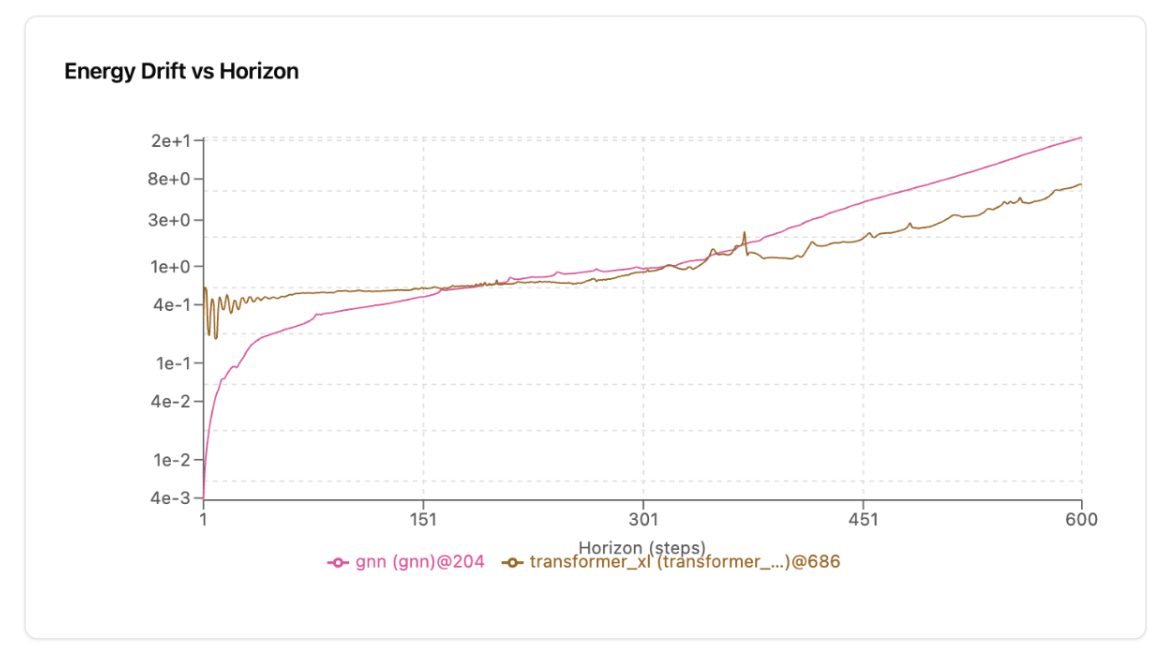
Sutton would be happy: the transformer now easily beats the GNN in both position error and energy drift stability even though its validation loss during training was higher than the GNN. The reason becomes obvious if we chart the aggregated energy drift (or position) errors for each time step of the validation trajectories. The GNN has lower error than the transformer up until roughly the end of the training horizon (10 seconds or 200 steps). After that point, the transformer wins.
The transformer likely benefits from the 8-position context buffer of past predictions that the GNN lacks. It also likely learned more general circuits from the 10 second training horizon that it uses to predict beyond it with lower error. So did it learn the actual underlying dynamics? Or is it using better heuristics and memorization to extrapolate beyond 10 seconds? One way to find out is by looking for predictions that obviously violate physics. It turns out they’re not hard to find. First, let’s look at an example with initial conditions (masses, velocities, positions) that are in the same distribution as the training trajectories:
The GNN predicts orbiting blue/green bodies but doesn’t track the ground truth. It keeps the red body on course but then breaks physics and veers it away from the other bodies around the 20 second mark. The transformer has finally learned the pairwise gravitational dynamics. The blue and green bodies correctly orbit one another but their orbit decays and like the GNN, doesn’t track the ground truth. The transformer’s physics-violating prediction happens around 18s with the red body when it suddenly veers away from the other bodies.
The deviation is subtle and takes work to spot, but this example was sampled from the same distribution of initial conditions used to generate our training data. Physically impossible predictions are much easier to spot if we use different initial conditions:
The initial conditions here create a Sun-Earth-Moon system and roll out to the same 10 second time horizon used in training. There are no forces pushing the bodies outside of the initial plane, so our expectation is that the prediction stays close to the ground-truth plane. The GNN decays the Earth’s orbit immediately, sending it speeding towards the sun, but its predictions are planar-ish. The transformer on the other hand maintains the Earth’s orbit better (although not perfect), but pulls the Earth and Moon immediately off-plane, with the sun following shortly after.
The more-general transformer architecture needed 13x the parameters and 3x the data to eventually overtake the much smaller GNN when predicting full trajectories beyond the training time horizon. The right inductive priors bought the GNN all of that for free. The larger transformer finally learned to predict basic pairwise motion, but its victory isn’t complete. It’s learned an approximation of the dynamics that isn’t quite physics. Changing the initial conditions easily pushes the model into predicting physically impossible motion. The GNN doesn’t escape this pitfall either. The pairwise prior gives it the right symmetries in its representation, but it’s still free to take shortcuts on the trajectory itself and rely on non-physical heuristics.
Reasons for Optimism
So why aren’t there more AlphaFolds? Two reasons: first, at the frontiers of science, data is scarce and doesn’t come with explanations. Training models to predict raw observations is different from training them to predict text because text is a result of human understanding of the universe. AlphaFold succeeds in generalizing from a small quantity of observations in part because of carefully crafted inductive priors. But the benefits don’t stop with data efficiency: the right priors prevent the model from taking a shortcut and learning via localized heuristics or memorization.
This then leads to the second reason why there aren’t more AlphaFolds: just pumping endless observations (if we have them available) into general-purpose architectures like transformers doesn’t necessarily train them to learn the underlying mechanisms that explain the data. If models predict by heuristics or memorization, we can’t trust their predictions outside the training distribution.
Designing and training AlphaFold-style models isn’t easy. You need deep expertise in two domains: the target science domain (in its case, protein folding), and machine learning. But there are reasons to be optimistic. Owing to a small dataset and strong inductive priors, AlphaFold 2 cost on the order of $100k to train. Its training dataset was completely public. Unlike frontier LLMs, training AlphaFold-class models is within reach of groups with domain expertise but without billions in GPUs. In parallel, agentic coding reduces the barriers to experimenting and training specialized architectures5. Perhaps the next AlphaFold won’t come from a frontier lab, but from a few domain experts and a good coding agent, training a small model with the right inductive priors.
Thanks to Xiaoyu Miao for providing feedback for drafts of this essay.
Footnotes
-
A Journal of the First Voyage of Vasco da Gama, 1497–1499, translated and edited by E. G. Ravenstein (Hakluyt Society, 1898). Project Gutenberg. ↩
-
James Lind, A Treatise of the Scurvy, in Three Parts (1753). Smithsonian Libraries. ↩
-
Jordan Hoffmann et al., Training Compute-Optimal Large Language Models, DeepMind, 2022. arXiv
.15556. ↩ -
Siddhant M. Jayakumar et al., Multiplicative Interactions and Where to Find Them, ICLR 2020. OpenReview. ↩
-
An AI system to help scientists write expert-level empirical software, Google Research. research.google. ↩